Ockhams Formula (Option Valuations)

Ockham's Razor has often been interpreted as "when you have two competing theories that make exactly the same predictions, the simpler one is the better." In the case of option valuations, I have found Ockham's Formula (Gallacher) significantly more practical than Black Scholes for a couple of reasons:

1) Ockham's is much simpler to apply and offers very similar accuracy as BS for ATM (At The Money) options.

* While Ockham's is not explicitly able to estimate fair value of OTM (Out of The Money) options, BS estimates are wildly inaccurate.

2) Ockham's gives answers where BS fails for options near expiration.

Ockham's ATM Option valuation

ATMO = S * 0.5 *  MAD * SD
             = S * 0.5 * sqrt(2/pi) * SD
             = S * 0.4 * SD
             = S * 0.4 * V * sqrt(T/254)
             = S * V / 40

where
ATMO = ATM fair value option price
S = Underlying product value
V = Realized volatility
T = days until option expiration       

Ockham's Option decay estimate
It is similar to theta, except this is much more accurate near expiration.

D(t, T) = 100 * [1 - sqrt(t/T)]

where
D(t, T) = Decay as a % of option price up to time t
T = days until option expiration   
t = days from expiration

For example, between the 4th and 5th trading days until expiration, an option is expected to lose
100 * [1 - sqrt(4/5)] = 10.5573%

Option prices are more efficient than you think

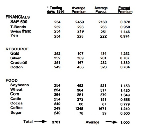
In The Options Edge, Gallagher looked at performance of (some interpolated) At-The-Money straddles between 15 futures options to determine whether options are indeed traded at a constant premium over future realized volatility, and concluded that they are most likely not.

In the experiment, he held and rolled front month straddles til expiration, back to back. In the last column, a ratio of 1 would mean the premium paid was exactly at fair value, if the ratio is below 1 the sellers made money, and vice versa.

Here are the findings:

 

We can see that at least for the year 1996, futures ATM Straddles were roughly traded at fair value.

My personal take on this

The normal distribution assumption off Black Scholes valuation is most likely off, significantly.

Empirically, blindly selling options does not generate a positive E(PnL), i.e. Expected Profit/Loss, particularly after transaction, hedging costs. At the same time, this also means buying volatility through options does not always carry a cost, this then in turn could lead to some very interesting trading strategies with very favorable risk/reward potentials.  

VIX Options Trading

Here's a look at the last 6 months of VIX options implied index against realized (index). Looks pretty easy to trade: buy low + sell high.

Candle Bars: VIX Index Implied Volatility Index
Blue Line: VIX Index Realized Volatility

*The last bar reaching infinity is obviously not a trade-able value.

Karen the (Incredibly Successful) Option Writer Interview

CBOE Skew Index

The implied skew index provides a point of reference for the S&P500 implied volatility smile.

Ever wonder if the far out-of-the-money (OTM) puts are relatively cheap or expensive with respect to at-the-money (ATM) options? Or how accurate it is at forecasting actual skewness of future SPX returns? Historical Skew Index Data is now freely available to answer these questions.

Here is a glimpse of the implied skew along with Realized Skew of SPX returns since 2001.

Options Deltas, Probability of expiring ITM

Delta is different from the probability of an option expiring In The Money (ITM); and here is the surprisingly simple mathematical proof.

According to Black Scholes,

where

σ = implied volatility

T = time to expiration

N(x) = cumulative normal distribution

Since σ and T are positive values, and that N(x) is a monotonically increasing function, it is logical that

 which then means

and we can see that the probability of a call expiring in the money must be less than its delta. The same logic applies to put options as well.

*The above also explains why delta of ATM calls are usually a bit greater than 0.5. 

From the math, it is apparent that this difference between delta and P(ITM) varies with respect to volatility and time to expiration, and becomes significant with far dated options in volatility contango.




 

Option delta off expected volatility (in Excel)

I think many of us have used the default delta values off implied volatility, and noticed that it can be off significantly when implied is way out of line against realized vol. This error makes the P&L of individual trades path dependent, and frequently hurt long volatility trades as delta becomes understated. A way reduce this error is to input realized vol for delta calculation, or 1 step better -> Expected Realized Vol.

Main advantage

The increased hedging accuracy would lower the volatility of individual trade returns, path dependance. It all goes toward achieving that positive EV:

EV = BSM(Realized Vol) - BSM(Implied) - transaction/hedging costs - implementation shortfalls
Where BSM() = Black Scholes Merton option valuation model.

Deriving delta

S -> Underlying value

K -> Strike price

r -> “Risk free” rate of return (often off 10year treasury)

V -> Expected realized volatility

T -> Option life with respect to year

We need to solve for d1 from the Black Scholes Merton model,

Then we can derive the “correct deltas”,

delta(Call) = N(d1)

delta(Put) = 1 – N(d1)

where N() = Position within the Standard Normal Distribution

Doing it in excel
So I used the latest SPY values for the example, and an arbitrary interest rate of 0.5% and realized vol of 12% (I didn't bother doing a forecast value since that's already covered in the earlier post).

Formulas:

We end up with

Delta hedged options, return estimate

So if we have a crude plan of delta hedging a long/short option position once a day, we'd like to know how far the underlying could go for us to make/lose money, as accurately as possible. Since gamma is associated with variance, and is a derivative of delta like acceleration off velocity; the return on a delta hedged options position is then like that of the distance formula from mechanical physics.

Distance formula: 
distance = (initial velocity)*(time) + (1/2)*(acceleration)*(time)^2

To translate this into a delta hedged options position, 

initial velocity -> delta
acceleration -> gamma
time -> change in the underlying

P&L of delta-hedged options

 









With a volatility forecast, the above gives us a pretty good idea of the position's EV (expected value).

Excel Data Analysis 3.2 (Volatility Forecasting off Linear Regression)

Today we look at forecasting RV( Realized Volatility) using linear regression for stock/index options trading. Generally speaking, an edge in estimating future realized volatility can be realized in units of vega off traded options; see Derman's paper, Trading Volatility, for details.

I'm still using the IYR data, and have updated the data (manually) up to Nov. 21, 2012.

Setting up linear regression

We need to match each realized volatility value from each day (row) with the future volatility, in this case I've picked the next 10 day. The calculation is exactly like the 20Day realized volatility, just instead of the past 20 days squared returns, we're using the coming 10days into the future. Logically, this column completes 10 trading days prior.

The future 10 day realized volatility is placed in the column F, RV.F10

 

Next we highlight the columns going from (E10, F10) down to the last row of RV.F10 at (E3127, F3127), and use the scatter plot.

Great, now the graph is up, we will have the 20Day RV on the X-axis, and RV.F10 on the Y-axis. Onto the regression fits, we right click the data on the chart and choose "add trendline". In the trendline menu, we want "Linear" type, and display "Equation on chart", "R-squared value on chart".

Remember that awesome Slope-Intercept Form, Y = mX + b, back from basic algebra? Well here it is again in the equation. As for the R-squared value, or Coefficient of Determination, the higher it is the better the equation represents the forecasting relationship.








Adaptive slope/intercept  values can be utilized as we update the excel worksheet day to day. This is so we wouldn't need to plot a graph every time for these values.

And we can see that the numbers are identical.











Great, now we can create a column, G, for realized volatility forecast values, I've named it FC(RV,10). Each day's next 10Day RV forecast would use the latest day's 20Day RV with the slope + intercept values.

So let's see how much of an edge this model offers us.

We can a column in H, for the day to day change in RV, named dRV. Then in columns I, named RV.u(FC) we can check each day's change in realized vol (dRV) if the previous day's forecast was higher than the previous day's ending RV. Vice versa for column J.

Note that in the if statement, I've used "" for value if false. Basically, it either gives the dRV value, or leaves it blank if false.

We can see from the average values that both directional forecasts had a slight edge, with the downside slightly more. Therefore in actual trading, I would not rely on this edge alone, but use it as a baseline bias for a feel of coming volatility.

Nikkei225 Realized Volatility at Different Hours

I was inspired by Jeff Augen to look up Nikkei 225 Index volatility between trading and off hours, and as expected a significant discrepancy is seem between them, with widely used close-to-close historical volatility at about the middle.

Why is this important?

It COULD be a way to exploit inefficiencies within option valuation, specifically vega.

Nikkei225 Realized Volatility since 1986
I used Nassim Taleb's method for volatility calculation using squared returns.

V.OC -  Annualized Historical Realized Volatility from open to close (Intraday)
V.G -  Annualized Historical Realized Volatility from the overnight Gap
V.C -  Annualized Historical Realized Volatility from close to close (conventional means)